Preparing a dataset

This page explains how to organise omic measurements and sample metadata, convert them into a MOSA dataset, and check the result before training. MOSA reads MuData stored as .h5mu files or .zarr directories. If your measurements are in separate tables, mosa convert aligns them by sample identifier and records which values are missing.

Each omic dataset is a view. Views can have different features and need not contain exactly the same samples: a sample measured in one view can have missing measurements in another. Sample identifiers must refer to the same biological samples across tables for the alignment to be meaningful.

Organise the input tables¶

Before conversion, process each dataset according to its omic type, origin, and quality. This may involve quality control, data cleaning, normalization, or harmonizing feature identifiers across sources. The appropriate operations depend on the data; conversion only aligns and stores the prepared measurements.

Arrange the processed measurements as one table per omic view, with a separate metadata table describing the samples. The commands below use data/gexp.csv, data/meth.csv, and data/metadata.csv; replace these paths with your own files.

Omic measurements¶

Arrange each view with features as rows and sample IDs as column headers. The first column contains feature identifiers; the remaining cells contain numeric measurements:

feature,SIDM00001,SIDM00002,SIDM00003
SLC7A11,6.42,5.11,7.30
CDKN2A,2.10,NaN,3.02

Use an empty cell or NaN for an unobserved measurement. Keep measured zeros as zero, since the model must distinguish an observed zero from missing data. Views do not need matching feature names unless you explicitly request a shared-feature intersection.

Supported table formats are .csv, .tsv, .txt, .tab, .parquet, and .pq; delimited files can use .gz, .bz2, .xz, or .zip compression. Tab-separated files use tabs between columns. For Parquet, retain feature identifiers as the table index or its first column.

Sample metadata¶

The metadata table has one row per sample. For example:

model_id,model_type,tissue
SIDM00001,source_A,Lung
SIDM00002,source_A,Breast
SIDM00003,source_B,Lung

model_id must be unique and match the sample IDs in the omic tables. model_type identifies the source or batch and is required even when all samples come from one source. It is used for source-stratified splitting and, by the MOSA VAE, for decoder conditioning and optional adversarial training. It does not select the integration model; that is the role of model.type in the experiment configuration.

tissue is optional for training. It supplies labels for tissue conditioning and contrastive training when enabled, and is required by mosa plot. Keep the labels consistent across datasets that will be trained or projected together.

To provide mutation conditionals, pass a binary features-by-samples table with --mutations data/mutations.csv. Each feature becomes a mutation_* metadata column. Mutation tables must already use the metadata's sample IDs. Missing mutation entries and samples absent from that table are filled with zero, so check that this treatment is appropriate for your data.

Convert the tables¶

Once the tables are ready, use mosa convert to name each view and provide its path:

mosa convert --conditionals data/metadata.csv \
  --view gexp:data/gexp.csv \
  --view meth:data/meth.csv \
  --output data/data.h5mu

The --conditionals argument supplies sample metadata. In each --view name:path argument, the name becomes the view identifier in the saved file, configuration, and reconstruction filenames. Choose names you can use consistently throughout the experiment.

Conversion preserves the supplied measurement values. It does not perform assay-specific normalization, scaling, or imputation. The VAE fits its own scaling and imputation using training samples; any preprocessing you perform beforehand must also respect the evaluation split when estimating statistics from the cohort.

Zarr is a storage format that divides arrays into compressed chunks. This allows lazy loading: reading only the chunks needed for an operation rather than loading the entire array into memory. To save the dataset in this format, replace the output argument with --output data/data.zarr --format zarr.

Alignment¶

By default, conversion retains samples that appear in the metadata and at least one view table, then sorts them by identifier. Samples found only in metadata or only in the omic tables are excluded. A retained sample absent from a view receives missing values for all features of that view.

If providers use different identifiers for the same samples, supply --id-map data/id-map.csv. This table maps source_id to the canonical model_id used in metadata. The mapping applies to omic tables; metadata and mutation tables must already use canonical IDs.

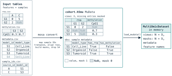
In this example, RNA identifiers A and C map to S1 and S3. Both views are aligned to S1, S2, S3; S4 is excluded because it appears only in metadata. The measured RNA zero retains a true mask entry, while missing measurements have false mask entries. The has_rna and has_methylation columns record which input tables contained each sample.

After conversion, mosa convert prints a summary in the terminal called the conversion report. It lists the number of samples retained and excluded, the feature count for each view, and how many samples appear in one, two, or more views.

Use this summary to check that conversion retained the cohort you intended. Samples excluded because they lack metadata or do not appear in any view table are counted separately. If more samples were excluded than expected, compare the identifiers in the metadata and omic tables for naming differences.

Combining files for one view¶

If an omic is distributed across several files, repeat its view name:

mosa convert --conditionals data/metadata.csv \
  --view gexp:data/gexp-source-a.csv \
  --view gexp:data/gexp-source-b.csv \
  --view meth:data/meth.csv \
  --output data/data.h5mu

MOSA combines the samples and retains the union of features within that view. Features absent from one file are missing for its samples. If a sample ID occurs twice within the combined view, conversion rejects the collision by default. Resolve duplicate or conflicting measurements before conversion; --on-collision first is available when retaining the first occurrence is the intended choice.

Filtering¶

Use conversion filters when the intended cohort excludes samples or requires a minimum amount of omic coverage:

These options select samples or features without changing retained measurements. Check the report after filtering to confirm the remaining cohort matches your intention.

File contents¶

Within the saved MuData object, each view stores measurements in X as samples × features, with an equally shaped Boolean mask layer. A true mask entry marks an observed measurement. Sample metadata is stored in .obs, along with mutation conditionals and has_<view> columns.

Each has_<view> column records whether a sample was included in the corresponding input table. For example, has_gexp is True when the sample ID appears as a column header in the gexp table, even if every measurement in that column is missing. The mask records availability at the measurement level: each sample–feature entry is True for an observed value and False for a missing value.

A sample included in the gexp table with no recorded measurements therefore has has_gexp = True, while its entire row in the saved gexp mask is False. The conversion report counts this sample as present in the input table. mosa inspect counts it as having no observed data in that view, so the two reported sample counts can differ.

Using a dataset prepared in Python¶

You can also create a MuData dataset in your own Python code, or use one saved by another tool. Before using that dataset with MOSA, check that it has the structure described above. mosa convert creates this structure automatically.

In a MuData object named mdata, mdata.obs is the shared sample metadata table, indexed by sample ID. Every view must contain those same sample IDs in the same order, so a given row refers to the same sample throughout the dataset. Each view also needs a Boolean observed-value mask in layers["mask"], with the same dimensions as its measurement matrix. The shared mdata.obs table must contain model_type, even when all samples have the same source label.

Add other sample annotations, such as tissue, as columns in mdata.obs. Avoid using mdata.obsm["<view name>"] for these annotations: MuData uses those entries to record which samples belong to each view.

Check the dataset before training¶

mosa inspect --input data/data.h5mu

Compare the reported sample IDs, view names, feature counts, value ranges, and missingness with your input tables. Check source-label counts as well: the training holdout needs at least two samples per source and enough samples for the requested fraction, while stratified cross-validation needs at least n_folds per source. Warnings about empty or approximately zero-valued views may indicate an input problem.

Use the reported view names in data.views and, for the VAE, in model.views. If a view should remain unscaled, list it in data.discrete_views. The VAE then retains observed values and fills missing entries with zero, but still uses squared-error reconstruction; marking a view as discrete does not introduce a discrete likelihood.

Once these checks pass, follow Training and projection to configure and fit the model. The convert reference lists all command options.